The Core computation on the software
The Software was designed to the be both simple to use by the available command line interface, and yet very fast on perfoming the power spectrum computation.
The speed is achieved by the union of 3 methods:
Keep in mind the pseudocode for the algorithm of the power computation:
1 2 3 4 5 6 7 8 9 10 11 12 13 14 15 16 17 18 19 | function PERIODOGRAM(T[N], F[M]) Input: T[N]: array with photon arrival times Input: F[M]: array with frequency spectrum for i = 0 to M − 1 do - compute Z2n power for each frequency for j = 0 to N − 1 do - compute phase for each photon arrival time ϕj = T[j] * F[i] ϕj = ϕj - ⌊ϕj⌋ sines[j] = SIN(2π * ϕj) cosines[j] = COS(2π * ϕj) end for sin = SUM(sines) cos = SUM(cosines) Z2n[j] = sin**2 + cos**2 end for Z2n[j] = Z2n * (2/LEN(T)) return Z2n end function |
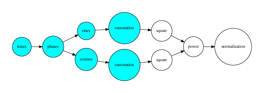
Each result on the power spectrum will be obtained by the computation of the following graph. There are two different subtrees on the computation graph, both can be executed in parallel on different threads.
Vectorization
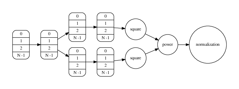
Besides the parallel threads, the operations on each blue node encapsulate the full range of the photon arrival times, therefore can be vectorized as shown on the following graph.
Parallel Loops
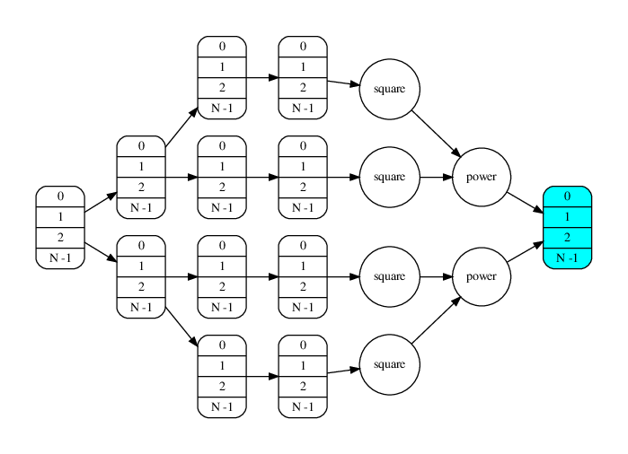
The resulting power spectrum will be the blue node on the following graph, that is the product of the parallel computation of many threads (according to the processor CPU) each of a different frequency graph.
Compilation
The process of compiling the Python source code into machine code (assembly x86) optimized for each function is achieved by the Numba JIT (just-in-time) compiler, with the available decorators for wrapping functions. Taking advantage of this process makes it easy to avoid the GIL (global interpreter lock) of the Python language.